MoveIt
A 2017 highlight reel for MoveIt, the ROS package that provides a high-level interface to OMPL and other motion planning packages.
Planning with constraints
OMPL has support for motion planning subject to hard constraints, including, but not limited to, Cartesian planning. In a 2019 paper in the International Journal of Robotics Research we describe how we have integrated prior motion planning approaches to planning with constraints in one framework that allows you to use any of the OMPL planners for constrained planning. The video below illustrates the main ideas. The examples in the videos are included as demo programs in the ompl/demos/constraint directory.
Manipulation Planning
An example of using OMPL on the PR2 from Willow Garage. The robot is asked to move the manipulate objects on the table. This demo is using ROS.
ROS-Industrial Consortium
ROS-Industrial aims to bring ROS to the industrial world. Path and motion planning, as provided by OMPL, are critical component of that. Below is brief overview of ROS-Industrial.
Real-time footstep planning for humanoid robots
Below is a video illustrating the results of using OMPL to plan footsteps for a humanoid. The work is described in detail in:
Nicolas Perrin and Olivier Stasse and Florent Lamiraux and Young J. Kim and Dinesh Manocha, Real-time footstep planning for humanoid robots among 3D obstacles using a hybrid bounding box, in Proc. IEEE Conf. on Robotics and Automation, 2012.
The focus is not so much on OMPL, but rather a new hybrid bounding box that allows the robot to step over obstacles.
Planning for a Car-Like Vehicle Using ODE
An example of using OMPL to plan for a robotic system simulated with ODE. The goal is for the yellow car to reach the location of the green box without hitting the red box. The computation is performed using KPIECE. For each computed motion plan, a representation of the exploration data structure (a tree of motions) is also shown.
Planning Using OMPL.app
Below are some rigid body motion planning problems and corresponding solutions found by OMPL.app. The planar examples use a kinematic car model.
Planning for Underactuated Systems in the Presence of Drift
In the game of Koules, there are a number of balls (called koules) flying in an orbit. The user controls a spaceship. At any time the user can do one of four things: coast, accelerate, turn left, or turn right. The ship and the koules are allowed to collide. The objective is for the ship to bounce all the koules out of the workspace. The user loses when the ship is bounced out of the workspace first. We have written a demo program that solves this game. The physics have been made significantly harder than in the original game. The movie below shows a solution path found by the Koules demo for 7 koules.
Class Project from COMP 450 on Path Optimization
In Fall 2010 OMPL was used for the first time in Lydia Kavraki's Algorithmic Robotics class. Students completed several projects. For their last project they could choose from several options. Linda Hill and Yu Yun worked on path optimization. The different optimization criteria considered they considered were path length and sum of discrete path curvature sum. Minimizing the former in shorter paths, minimizing the second results in smoother paths. They used two optimization techniques specific to paths / curves: B-spline interpolation and path hybridization. Path smoothing using B-spline interpolation is shown below on the left. In path hybridization a set of (approximate) solutions to a motion planning problem is given as input, cross-over points are computed, and a new optimized path composed of path segments is found. An example of path hybridization to minimize path length is shown below on the right. In both cases the paths were in SE(3); the figures show simply the R3 component.
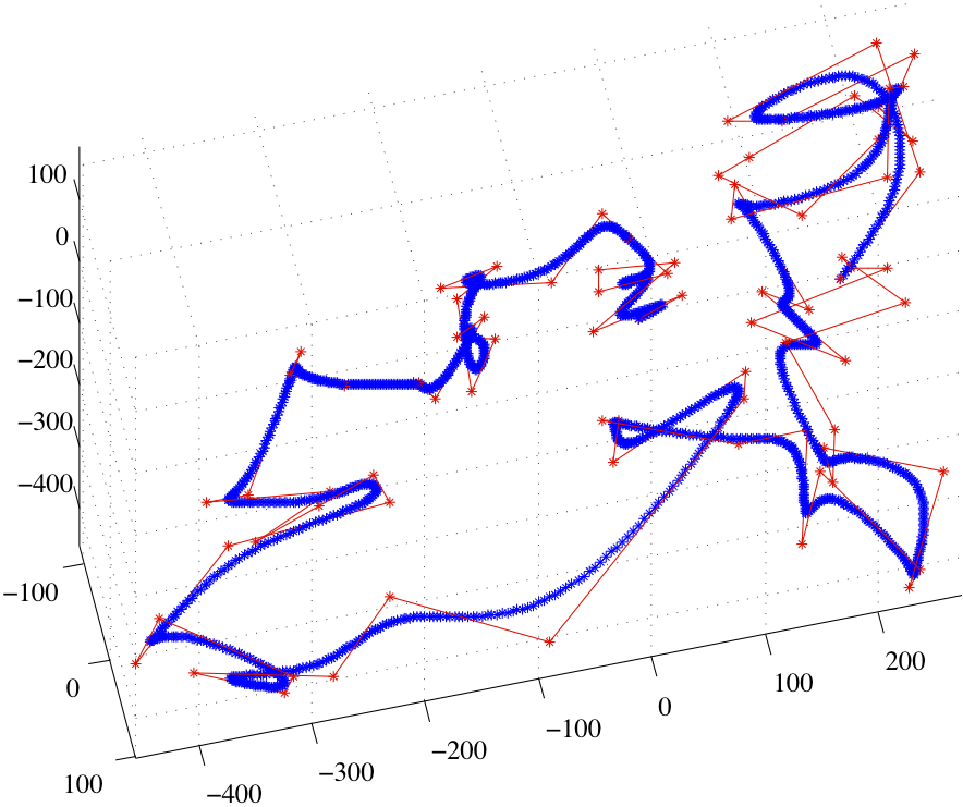
Path smoothing with B-splines. The input path is shown in red, the optimized output path is shown in blue.
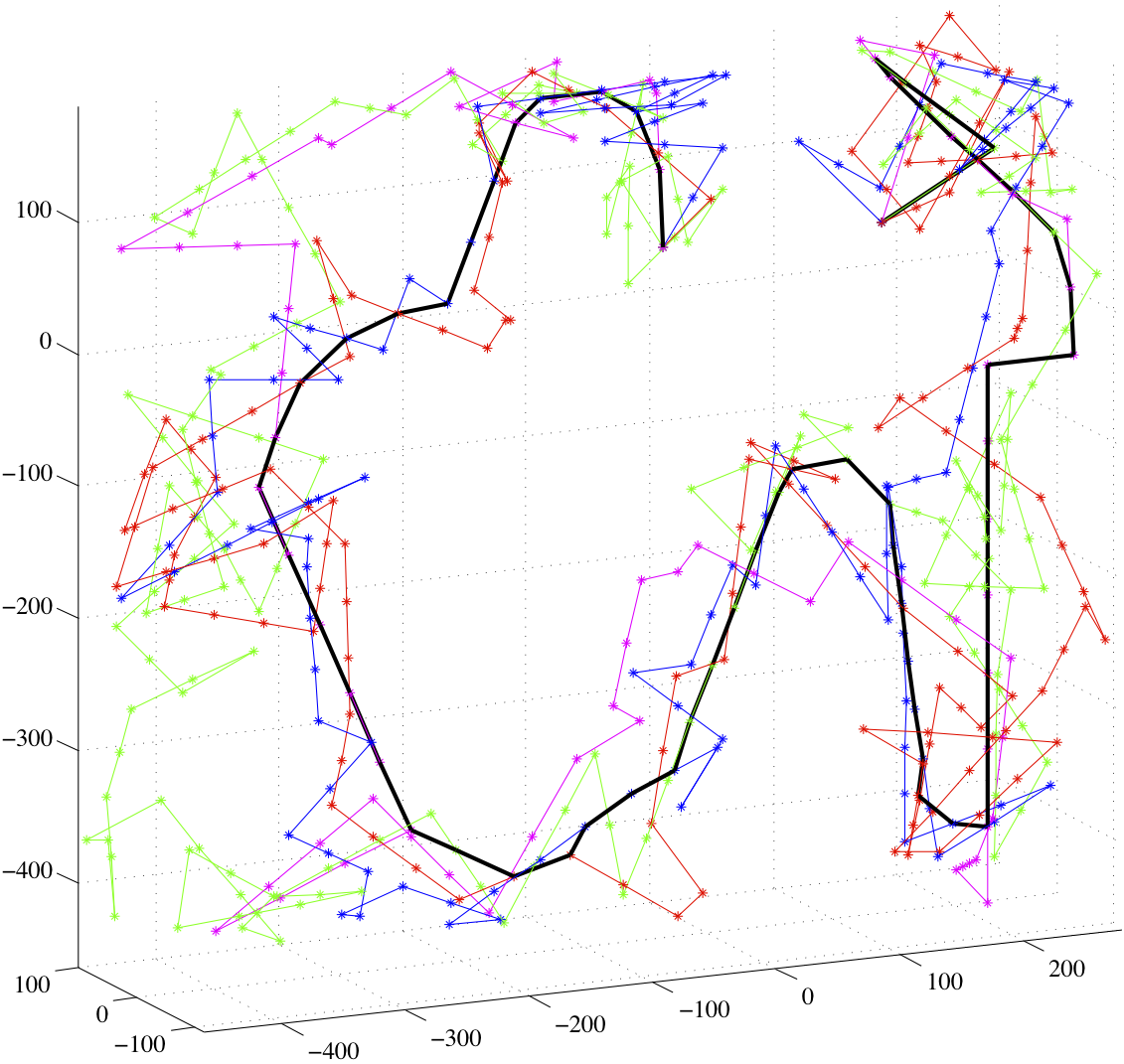
Path shortening using path hybridization. The colored paths are input, the solid black path is the optimized output path.