How to Benchmark Planners

Table of Contents

• Create a benchmark configuration file
• Writing benchmarking code
• Processing the benchmarking log file
• Sample benchmark results
• The benchmark logfile format
• The benchmark database schema

OMPL contains a ompl::Benchmark class that facilitates solving a motion planning problem repeatedly with different parameters, different planners, different samplers, or even differently configured versions of the same planning algorithm. Below, we will describe how you can use this class.

For interactive visualization of benchmark databases, please see plannerarena.org.

Create a benchmark configuration file

OMPL.app contains a command line program called ompl_benchmark, that can read a text based configuration file using an ini style format with key/value pairs. This is the same format that can be read and saved with the OMPL.app GUI. The GUI ignores the settings related to benchmarking. However, it is often convenient to create an initial configuration with the GUI and add the benchmark settings with a text editor. Currently the base functionality of the ompl_benchmark program only applies to geometric planning in SE(2) and SE(3) and kinodynamic planning for certain systems, but the program can be extended by the user to other types of planning problems.

There are a number of required parameters necessary to define the problem. These exist under the “**[problem]**” heading:

• name: An identifying name for the problem to be solved.
• robot: The path to a mesh file describing the geometry of the robot.
• start.[x|y|z|theta], start.axis.[x|y|z]: Values describing the start state of the robot. In 2D, the orientation is specified with just start.theta, while in 3D the axis-angle orientation is used.
• goal.[x|y|z|theta], goal.axis.[x|y|z]: Values describing the goal state of the robot.

The following parameters are optional under the “**[problem]**” heading:

• world: The path to a mesh file describing the geometry of the environment. If unspecified, it is assumed that the robot operates in an empty workspace.
• objective: Some planners in OMPL can optimize paths as a function of various optimization objective. The objective parameter can be set to length, max_min_clearance, or mechanical_work, to minimize path length, maximize minimum clearance along the path, or mechanical work of the path, respectively. If unspecified, it is assumed the objective is length.
• objective.threshold: If an objective is specified, you can optionally also specify the objective.threshold, which causes optimizing planners to terminate once they find a path with cost better than the specified threshold (a real-valued number). If unspecified, the best possible value is chosen for a threshold (e.g., for path length that would be 0), so that optimizing planners will try to find a shortest possible path.
• control: There a few built-in kinodynamic systems in OMPL.app. The control parameter can be set to kinematic_car, dynamic_car, blimp, and quadrotor. If unspecified, rigid-body planning is assumed. Beware that kinodynamic planning is much harder than rigid-body planning.
• sampler: This parameter specified the sampler to be used by the planner. The following samplers are available: uniform, gaussian, obstacle_based, max_clearance. If unspecified, the uniform sampler is used.
• volume.[min|max].[x|y|z]: It is sometimes necessary to specify the bounds of the workspace. Without any specification, OMPL.app assumes a tight bounding box around the environment (if specified) and the start and goal states, but depending on the environment this may not be a good assumption.

Parameters relating to benchmarking must be declared under the “**[benchmark]**” heading:

• time_limit: The amount of time (seconds) for each plan computation.
• mem_limit: The maximum amount of memory (MB) for each planner. Memory measurements are not very accurate, so it is recommended to set this to a very large value.
• run_count: The number of times to repeat the experiment for each planner.
• output: Output directory where the benchmark log file will be saved. This parameter is optional; by default the log file is saved in the same directory as the configuration file.
• save_paths: This optional parameter can be set to none, all, or shortest to save no solution paths (the default value), all solution paths (including approximate solutions), or the shortest exact solution for each planner, respectively. These paths can then be “played back” in the OMPL.app GUI.

The last required element to specify are the planners to benchmark. These are specified under the “**[planner]**” heading. The following planners are valid for geometric benchmarking: kpiece, bkpiece, lbkpiece, est, sbl, prm, lazyprm, lazyprmstar, rrt, rrtconnect, lazyrrt, rrtstar, lbtrrt, trrt, spars, spars2, stride, pdst, fmt, and aps. The following planners are valid for kinodynamic planning (i.e., when the control parameter is set): kpiece, rrt, est, pdst, sycloprrt, and syclopest.

An example of a minimal SE(2) configuration comparing the rrt and est planners is given below:

[problem]
name=my_benchmark_problem
robot=my_robot_mesh.dae
start.x=0.0
start.y=0.0
start.theta=0.0
goal.x=1.0
goal.y=1.0
goal.theta=0.0
 
[benchmark]
time_limit=10.0
mem_limit=1000.0
run_count = 3
 
[planner]
est=
rrt=

Any parameter defined by these planners may also be configured for the benchmark. For example, the geometric::RRT planner defines two parameters, “range” and “goal_bias”, both real valued. The default values can be changed under the “planner” heading in the following manner:

• rrt.range=50.0
• rrt.goal_bias=0.10

There are many other optional parameters that can be specified or changed. The ompl_benchmark executable takes advantage of the ompl::base::ParamSet class, and uses this functionality to set any parameter defined in the file. If a class exposes a parameter, chances are that it is possible to tune it via the config file. OMPL.app provides two example configuration files inside of the benchmark directory, example.cfg and example_complex.cfg showing the configuration of many of these optional parameters.

It is possible to create multiple instances of the same planner and configure each differently. This code, for example, creates two instances of rrtconnect with different values for its range parameter:

rrtconnect=
rrtconnect.range=100
rrtconnect=
rrtconnect.range=200

Moreover, the problem settings can be changed between different planner instances. Below, some of the problem settings are changed for the second instance of kpiece.

kpiece=
kpiece=
# increase the size of the projection by a specific factor, in every dimension
problem.projection.cellsize_factor = 4.0
# specify a different sampler
problem.sampler=obstacle_based

When using multiple planner instances, a useful parameter is “name”, as it can be used to rename a planner. For example, two instances of geometric::PRM can be created but named differently. Having different names is useful when processing the resulting log data using the benchmark script.

prm=
problem.sampler=uniform
prm.name=uniprm
prm=
problem.sampler=obstacle_based
prm.name=obprm

Finally, to execute the benchmark configuration file, simply run the ompl_benchmark executable in the OMPL.app bin directory, and supply the path to the config file as the first argument.

Writing benchmarking code

Benchmarking a set of planners on a specified problem using the Benchmark class in your own code is a simple task in OMPL. The steps involved are as follows:

• Configure the benchmark problem using ompl::geometric::SimpleSetup or ompl::control::SimpleSetup
• Create a ompl::Benchmark object that takes the problem as input
• Optionally, specify some parameters for the benchmark object using ompl::Benchmark::addExperimentParameter, which is useful when aggregating benchmark results over parametrized benchmarks.
• Add one or more planners to the benchmark
• Optionally add events to be called before and/or after the execution of a planner
• Run the benchmark problem a specified number of times, subject to specified time and memory limits

The following code snippet shows you how to do this. We will start with some initial code that you have probably already used:

#include "ompl/tools/benchmark/Benchmark.h"
 
// A function that matches the ompl::base::PlannerAllocator type.
// It will be used later to allocate an instance of EST
ompl::base::PlannerPtr myConfiguredPlanner(const ompl::base::SpaceInformationPtr &si)
{
    geometric::EST *est = new ompl::geometric::EST(si);
    est->setRange(100.0);
    return ompl::base::PlannerPtr(est);
}
 
// Create a state space for the space we are planning in
ompl::geometric::SimpleSetup ss(space);
 
// Configure the problem to solve: set start state(s)
// and goal representation
// Everything must be set up to the point ss.solve()
// can be called. Setting up a planner is not needed.

Benchmarking code starts here:

// First we create a benchmark class:
ompl::tools::Benchmark b(ss, "my experiment");
 
// Optionally, specify some benchmark parameters (doesn't change how the benchmark is run)
b.addExperimentParameter("num_dofs", "INTEGER", "6")
b.addExperimentParameter("num_obstacles", "INTEGER", "10")
 
// We add the planners to evaluate.
b.addPlanner(base::PlannerPtr(new geometric::KPIECE1(ss.getSpaceInformation())));
b.addPlanner(base::PlannerPtr(new geometric::RRT(ss.getSpaceInformation())));
b.addPlanner(base::PlannerPtr(new geometric::SBL(ss.getSpaceInformation())));
b.addPlanner(base::PlannerPtr(new geometric::LBKPIECE1(ss.getSpaceInformation())));
// etc
 
// For planners that we want to configure in specific ways,
// the ompl::base::PlannerAllocator should be used:
b.addPlannerAllocator(std::bind(&myConfiguredPlanner, std::placeholders::_1));
// etc.
 
// Now we can benchmark: 5 second time limit for each plan computation,
// 100 MB maximum memory usage per plan computation, 50 runs for each planner
// and true means that a text-mode progress bar should be displayed while
// computation is running.
ompl::tools::Benchmark::Request req;
req.maxTime = 5.0;
req.maxMem = 100.0;
req.runCount = 50;
req.displayProgress = true;
b.benchmark(req);
 
// This will generate a file of the form ompl_host_time.log
b.saveResultsToFile();

Adding callbacks for before and after the execution of a run is also possible:

// Assume these functions are defined
void optionalPreRunEvent(const base::PlannerPtr &planner)
{
    // do whatever configuration we want to the planner,
    // including changing of problem definition (input states)
    // via planner->getProblemDefinition()
}
 
void optionalPostRunEvent(const base::PlannerPtr &planner, tools::Benchmark::RunProperties &run)
{
    // do any cleanup, or set values for upcoming run (or upcoming call to the pre-run event).
 
    // adding elements to the set of collected run properties is also possible;
    // (the added data will be recorded in the log file)
 
    run["some extra property name INTEGER"] = "some value";
    // The format of added data is string key, string value pairs,
    // with the convention that the last word in string key is one of
    // REAL, INTEGER, BOOLEAN, STRING. (this will be the type of the field
    // when the log file is processed and saved as a database).
    // The values are always converted to string.
}
 
// After the Benchmark class is defined, the events can be optionally registered:
b.setPreRunEvent(std::bind(&optionalPreRunEvent, std::placeholders::_1));
b.setPostRunEvent(std::bind(&optionalPostRunEvent, std::placeholders::_1, std::placeholders::_2));

Processing the benchmarking log file

Once the C++ code computing the results has been executed, a log file is generated. This contains information about the settings of the planners, the parameters of the problem tested on, etc. To visualize this information, we provide a script that parses the log files:

ompl/scripts/ompl_benchmark_statistics.py logfile.log -d mydatabase.db

This will generate a SQLite database containing the parsed data. If no database name is specified, the named is assumed to be benchmark.db. Once this database is generated, we can visualize the results. The recommended way is to upload the database to Planner Arena and navigate through the different plots. Planner Arena can also be run locally with the plannerarena script (requires R to be installed). Alternatively, you can also produce some basic plots with ompl_benchmark_statistics.py like so:

ompl/scripts/ompl_benchmark_statistics.py -d mydatabase.db -p boxplot.pdf

This will generate a series of plots, one for each of the attributes described below, showing the results for each planner. Below we have included some sample benchmark results.

If you would like to process the data in different ways, you can generate a dump file that you can load in a MySQL database:

ompl/scripts/ompl_benchmark_statistics.py -d mydatabase.db -m mydump.sql

For more details on how to use the benchmark script, see:

scripts/ompl_benchmark_statistics.py --help

Collected benchmark data for each experiment:

• name: name of experiment (optional)
• totaltime: the total duration for conducting the experiment (seconds)
• timelimit: the maximum time allowed for every planner execution (seconds)
• memorylimit: the maximum memory allowed for every planner execution (MB)
• hostname: the name of the host on which the experiment was run
• date: the date and time when the experiment was started

Collected benchmark data for each planner execution:

• time: (real) the amount of time spent planning, in seconds
• memory: (real) the amount of memory spent planning, in MB. Note: this may be inaccurate since memory is often freed in a lazy fashion
• solved: (boolean) flag indicating whether the planner found a solution. Note: the solution can be approximate
• approximate solution: (boolean) flag indicating whether the found solution is approximate (does not reach the goal, but moves towards it)
• solution difference: (real) if the solution is approximate, this is the distance from the end-point of the found approximate solution to the actual goal
• solution length: (real) the length of the found solution
• solution smoothness: (real) the smoothness of the found solution (the closer to 0, the smoother the path is)
• solution clearance: (real) the clearance of the found solution (the higher the value, the larger the distance to invalid regions)
• solution segments: (integer) the number of segments on the solution path
• correct solution: (boolean) flag indicating whether the found solution is correct (a separate check is conducted). This should always be true.
• correct solution strict: (boolean) flag indicating whether the found solution is correct when checked at a finer resolution than the planner used when validating motion segments. If this is sometimes false it means that the used state validation resolution is too high (only applies when using ompl::base::DiscreteMotionValidator).
• simplification time: (real) the time spend simplifying the solution path, in seconds
• simplified solution length: (real) the length of the found solution after simplification
• simplified solution smoothness: (real) the smoothness of the found solution after simplification (the closer to 0, the smoother the path is)
• simplified solution clearance: (real) the clearance of the found solution after simplification (the higher the value, the larger the distance to invalid regions)
• simplified solution segments: (integer) the number of segments on solution path after simplification
• simplified correct solution: (boolean) flag indicating whether the found solution is correct after simplification. This should always be true.
• simplified correct solution strict: (boolean) flag indicating whether the found solution is correct after simplification, when checked at a finer resolution.
• graph states: (integer) the number of states in the constructed graph
• graph motions: (integer) the number of edges (motions) in the constructed graph
• valid segment fraction: (real) the fraction of segments that turned out to be valid (using ompl::base::MotionValidator) out of all the segments that were checked for validity
• more planner-specific properties

Planning algorithms can also register callback functions that the Benchmark class will use to measure progress properties at regular intervals during a run of the planning algorithm. Currently only RRT* uses this functionality. The RRT* constructor registers, among others, a function that returns the cost of the best path found so far:

addPlannerProgressProperty("best cost REAL", std::bind(&RRTstar::getBestCost, this));

With the Benchmark class one can thus measure how the cost is decreasing over time. The ompl_benchmark_statistics.py script will automatically generate plots of progress properties as a function of time.

Sample benchmark results

Below are sample results for running benchmarks for two example problems: the “cubicles” environment and the “Twistycool” environment. The complete benchmarking program (SE3RigidBodyPlanningBenchmark.cpp), the environment and robot files are included with OMPL.app, so you can rerun the exact same benchmarks on your own machine. See the gallery for visualizations of sample solutions to both problems. The results below were run on a recent model Apple MacBook Pro (2.66 GHz Intel Core i7, 8GB of RAM). It is important to note that none of the planner parameters were tuned; all benchmarks were run with default settings. From these results one cannot draw any firm conclusions about which planner is “better” than some other planner.

These are the PDF files with plots as generated by the ompl_benchmark_statistics.py script:

• The “cubicles” problem with default settings
• The “Twistycool” problem with default settings

The plots show comparisons between ompl::geometric::RRTConnect, ompl::geometric::RRT, ompl::geometric::BKPIECE1, ompl::geometric::LBKPIECE1, ompl::geometric::KPIECE1, ompl::geometric::SBL, ompl::geometric::EST, and ompl::geometric::PRM. Each planner is run 500 times with a 10 second time limit for the cubicles problem for each sampling strategy, while for the Twistycool problem each planner is run 50 times with a 60 second time limit.

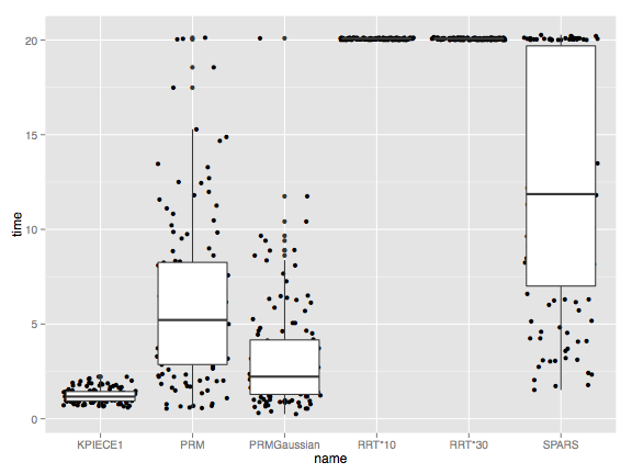
For integer and real-valued measurements the script will compute box plots. For example, here is the plot for the real-valued attribute time for the cubicles environment:

For boolean measurements the script will create bar charts with the percentage of true values. For example, here is the plot for the boolean attribute solved for the Twistycool environment, a much harder problem:

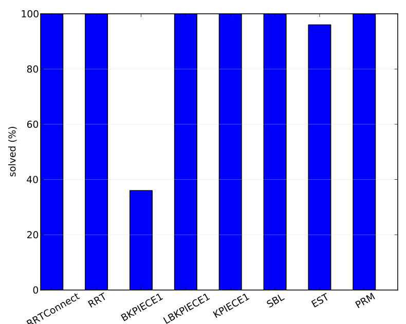
Whenever measurements are not always available for a particular attribute, the columns for each planner are labeled with the number of runs for which no data was available. For instance, the boolean attribute correct solution is not set if a solution is not found.

The benchmark logfile format

The benchmark log files have a pretty simple structure. Below we have included their syntax in Extended Backus-Naur Form. This may be useful for someone interested in extending other planning libraries with similar logging capabilities (which would be helpful in a direct comparison of the performance of planning libraries). Log files in this format can be parsed by ompl_benchmark_statistics.py (see next section).

logfile               ::= preamble planners_data;
preamble              ::= [version] experiment [exp_property_count exp_properties] hostname date setup [cpuinfo]
                          random_seed time_limit memory_limit [num_runs]
                          total_time [num_enums enums] num_planners;
version               ::= library_name " version " version_number EOL;
experiment            ::= "Experiment " experiment_name EOL;
exp_property_count    ::= int " experiment properties" EOL;
exp_properties        ::= exp_property | exp_property exp_properties;
exp_property          ::= name property_type "=" num EOL;
hostname              ::= "Running on " host EOL;
date                  ::= "Starting at " date_string EOL;
setup                 ::= multi_line_string;
cpuinfo               ::= multi_line_string;
multi_line_string     ::= "<<<|" EOL strings "|>>>" EOL;
strings               ::= string EOL | string EOL strings
random_seed           ::= int " is the random seed" EOL;
time_limit            ::= float " seconds per run" EOL;
memory_limit          ::= float " MB per run" EOL;
num_runs              ::= int " runs per planner" EOL;
total_time            ::= float " seconds spent to collect the data" EOL;
num_enums             ::= num " enum type" EOL;
enums                 ::= enum | enum enums;
enum                  ::= enum_name "|" enum_values EOL;
enum_values           ::= enum_value | enum_value "|" enum_values;
num_planners          ::= int " planners" EOL;
planners_data         ::= planner_data | planner_data planners_data;
planner_data          ::= planner_name EOL int " common properties" EOL
                          planner_properties int " properties for each run" EOL
                          run_properties int " runs" EOL run_measurements
                          [int "progress properties for each run" EOL
                          progress_properties int " runs" EOL
                          progress_measurements] "." EOL;
planner_properties    ::= "" | planner_property planner_properties;
planner_property      ::= property_name " = " property_value EOL;
run_properties        ::= property | property run_properties;
progress_properties   ::= property | property progress_properties;
property              ::= property_name " " property_type EOL;
property_type         ::= "BOOLEAN" | "INTEGER" | "REAL";
run_measurements      ::= run_measurement | run_measurement run_measurements;
run_measurement       ::= data "; " | data "; " run_measurement;
data                  ::= num | "inf" | "nan" | "";
progress_measurements ::= progress_measurement EOL
                         | progress_measurement EOL progress_measurements;
progress_measurement  ::= prog_run_data | prog_run_data ";" progress_measurement;
prog_run_data         ::= data "," | data "," prog_run_data;

Here, EOL denotes a newline character, int denotes an integer, float denotes a floating point number, num denotes an integer or float value and undefined symbols correspond to strings without whitespace characters. The exception is property_name which is a string that can have whitespace characters. It is also assumed that if the log file says there is data for k planners that that really is the case (likewise for the number of run measurements and the optional progress measurements).

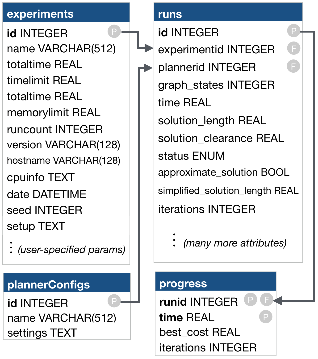
The benchmark database schema

The benchmark database schema

The ompl_benchmark_statistics.py script can produce a series of plots from a database of benchmark results, but in many cases you may want to produce your own custom plots. For this it useful to understand the schema used for the database. There are five tables in a benchmark database:

• experiments. This table contains the following information:
  • id: an ID used in the runs table to denote that a run was part of a given experiment.
  • name: name of the experiment.
  • totaltime: total duration of the experiment in seconds.
  • timelimit: time limit for each individual run in seconds.
  • memorylimit: memory limit for each individual run in MB.
  • runcount: the number of times each planner configuration was run.
  • version: the version of OMPL that was used.
  • hostname: the host name of the machine on which the experiment was performed.
  • cpuinfo: CPU information about the machine on which the experiment was performed.
  • date: the date on which the experiment was performed.
  • seed: the random seed used.
  • setup: a string containing a “print-out” of all the settings of the SimpleSetup object used during benchmarking.
• plannerConfigs. There are a number of planner types (such as PRM and RRT), but each planner can typically be configured with a number of parameters. A planner configuration refers to a planner type with specific parameter settings. The plannerConfigs table contains the following information:
  • id: an ID used in the runs table to denote that a given planner configuration was used for a run.
  • name: the name of the configuration. This can be just the planner name, but when using different parameter settings of the same planner it is essential to use more specific names.
  • settings: a string containing a “print-out” of all the settings of the planner.
• enums: This table contains description of enumerate types that are measured during benchmarking. By default there is only one such such type defined: ompl::base::PlannerStatus. The table contains the following information:
  • name: name of the enumerate type (e.g., “status”).
  • value: numerical value used in the runs
  • description: text description of each value (e.g. “Exact solution,” “Approximate solution,” “Timeout,” etc.)
• runs. The runs table contains information for every run in every experiment. Each run is identified by the following fields:
  • id: ID of the run
  • experimentid: ID of the experiment to which this run belonged.
  • plannerid: ID of the planner configuration used for this run.
  In addition, there will be many benchmark statistics. None are required, but the OMPL planners all report the properties described above such as time, memory, solution length, simplification time, etc. It is possible that not all planners report the same properties. In that case, planners that do not report such properties will have NULL values in the corresponding fields.
• progress. Some planners (such as RRT*) can also periodically report properties during a run. This can be useful to analyze the convergence or growth rate. The progress table contains the following information:
  • runid: the ID of the run for which progress data was tracked.
  • time: the time (in sec.) at which the property was measured.
  The actual properties stored depend on the planner, but in the case of RRT* it stores the following additional fields:
  • iterations: the number of iterations.
  • collision_checks: the number of collision checks (or, more precisely, the number state validator calls).
  • best_cost: the cost of the best solution found so far.

Using SQL queries one can easily select a subset of the data or compute joins of tables. Consider the following snippet of R code:

library("ggplot2")
library("RSQLite")
con <- dbConnect(dbDriver("SQLite"), "benchmark.db")
 
# read data
runs <- dbGetQuery(con, "SELECT REPLACE(plannerConfigs.name,'geometric_','') AS name, runs.* FROM plannerConfigs INNER JOIN runs ON plannerConfigs.id = runs.plannerid")
progress <- dbGetQuery(con, "SELECT REPLACE(plannerConfigs.name,'geometric_','') AS name, progress.* FROM plannerConfigs INNER JOIN runs INNER JOIN progress ON plannerConfigs.id=runs.plannerid AND runs.id=progress.runid")
 
# plot some data
pdf('plots.pdf', width=8, height=6)
qplot(name, time, data=runs, geom=c("jitter","boxplot"))
qplot(time, best_cost, data=progress, alpha=I(1/2), colour=name, geom=c("point", "smooth"))
 
dev.off()
dbDisconnect(con)

For a small database with 1 experiment (the “cubicles” problem from OMPL.app) and 5 planner configurations we then obtain the following two plots:

Time to find a solution. Note that that RRT* does not terminate because it keeps trying to find a more optimal solution.

Length of shortest path found after a given number of seconds. Only RRT* currently uses progress properties. Although the variability among individual runs is quite high, one can definitely tell that different parameter settings (for the range in this case) lead to statistically significant different behavior.

Note

Similar code is used for Planner Arena, a web site for interactive visualization of benchmark databases. The Planner Arena code is part of the OMPL source. Instructions for running Planner Arena locally can be found here.