Defining a constrained motion planning problem is easy and very similar to defining an unconstrained planning problem. The primary difference is the need to define a constraint, and the use of a constrained state space, which wraps around an ambient state space. In this example, we will walk through defining a simple constrained planning problem: a point in \(\mathbb{R}^3\) that is constrained to be on the surface of a sphere, giving a constraint function \(f(q) = \lVert q \rVert - 1\). This is very similar to the problem defined by the demo ConstrainedPlanningSphere.

Defining the Constraint

First, let's define our constraint class. Constraints must inherit from the base class ompl::base::Constraint. Primarily, the function ompl::base::Constraint::function() must be implemented by any concrete implementation of a constraint. A bare-bones version of the sphere constraint we gave above might look like this:

// Constraints must inherit from the constraint base class. By default, a
// numerical approximation to the Jacobian of the constraint function is computed
// using a central finite difference.
class Sphere : public ob::Constraint
{
public:
    // ob::Constraint's constructor takes in two parameters, the dimension of
    // the ambient state space, and the dimension of the real vector space the
    // constraint maps into. For our sphere example, as we are planning in R^3, the
    // dimension of the ambient space is 3, and as our constraint outputs one real
    // value the second parameter is one (this is also the co-dimension of the
    // constraint manifold).
    Sphere() : ob::Constraint(3, 1)
    {
    }
 
    // Here we define the actual constraint function, which takes in some state "x"
    // (from the ambient space) and sets the values of "out" to the result of the
    // constraint function. Note that we are implementing `function` which has this
    // function signature, not the one that takes in ompl::base::State.
    void function(const Eigen::Ref<const Eigen::VectorXd> &x, Eigen::Ref<Eigen::VectorXd> out) const override
    {
        // The function that defines a sphere is f(q) = || q || - 1, as discussed
        // above. Eigen makes this easy to express:
        out[0] = x.norm() - 1;
    }
};

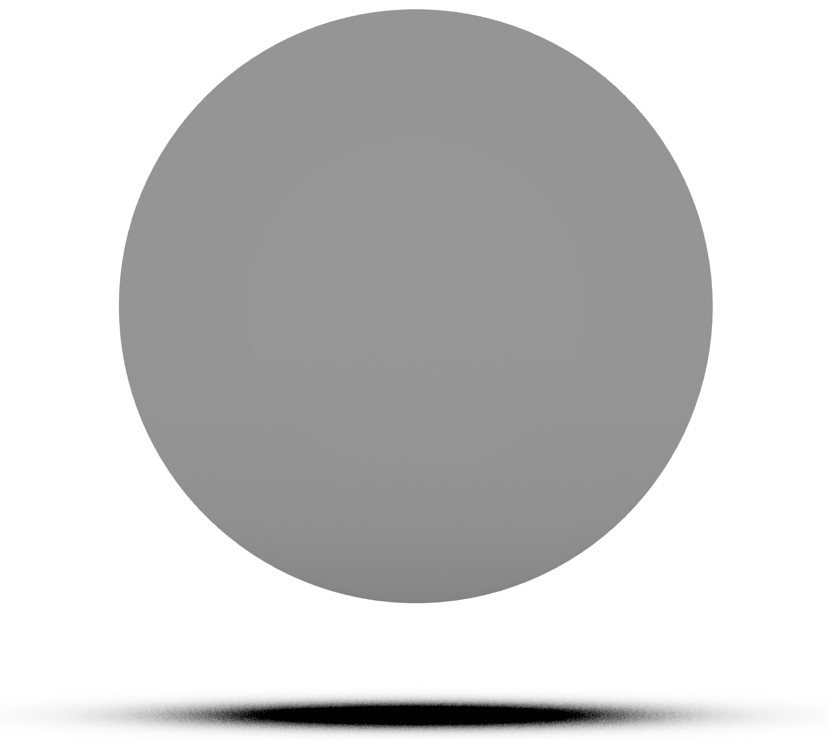
We now have a constraint function that defines a sphere in \(\mathbb{R}^3\)! We can visualize the constraint simply as a sphere in \(\mathbb{R}^3\), shown below.

Now we can use this constraint to define a constrained state space.

Constraint Jacobian

However, we can do better. We would like to include an analytical Jacobian for our constraint function, so that planning more efficient. Either we can compute this by hand, or we can use some symbolic solver (e.g., ConstraintGeneration.py shows how to do this with SymPy). Either way, we add to our class the function to compute the Jacobian:

// Implement the Jacobian of the constraint function. The Jacobian for the
// constraint function is an matrix of dimension equal to the co-dimension of the
// constraint by the ambient dimension (in this case, 1 by 3). Similar to
// `function` above, we implement the `jacobian` method with the following
// function signature.
void Sphere::jacobian(const Eigen::Ref<const Eigen::VectorXd> &x, Eigen::Ref<Eigen::MatrixXd> out) const override
{
    out = x.transpose().normalized();
}

In general, it is highly recommended that you provide an analytic Jacobian for a constrained planning problem, especially for high-dimensional problems.

Projection

One of the primary features of ompl::base::Constraint is the projection function, ompl::base::Constraint::project(). This function takes as input a potential constraint unsatisfying state and maps it onto the constraint manifold, generating a constraint satisfying state. By default, ompl::base::Constraint::project() implements a Newton's method which performs well in most circumstances.

However, it is possible to override this method with your own projection routine. For example, in the case of our sphere, it could simply normalize the state, placing it on the sphere. Another example would be to use inverse kinematics for a complex robot manipulator.

Constraint Parameters

ompl::base::Constraint affords a two parameters that affect performance. The first is tolerance, which can be set with ompl::base::Constraint::setTolerance(), or via the constructor. Using the constructor, our Sphere class could like like this:

...
    // Set ambient and constraint dimension, along with tolerance (1e-3, in this case).
    Sphere() : ob::Constraint(3, 1, 1e-3)
...

tolerance is used in ompl::base::Constraint::project() to determine when a state satisfies the constraints, and in ompl::base::Constraint::isSatisfied() for the same purpose. For problems that afford lower tolerances (e.g., highly compliant robots), tolerance can be lowered. Lower tolerance values generally simplifies the planning problem, as it is easier to satisfy constraints.

The second is maxIterations, which can be set with ompl::base::Constraint::setMaxIterations(). maxIterations is used in ompl::base::Constraint::project() to limit the number of iterations the projection routine uses, in the case that a satisfying configuration cannot be found. It might be necessary to adjust this value for particularly easy or hard constraint functions to satisfy (decreasing and increasing iterations respectively).

Defining the Constrained State Space

Ambient State Space

Before we can define a constrained state space, we need to define the ambient state space \(\mathbb{R}^3\).

// Create the ambient space state space for the problem.
auto rvss = std::make_shared<ob::RealVectorStateSpace>(3);
 
// Set bounds on the space.
ob::RealVectorBounds bounds(3);
bounds.setLow(-2);
bounds.setHigh(2);
 
rvss->setBounds(bounds);

The ambient space is the space over which the constraint is defined, and is used by our constrained state space.

Constraint Instance

We then need to create an instance of our constraint:

// Create our sphere constraint.

auto constraint = std::make_shared<Sphere>();

The constraint instance is used by our constrained state space.

Constrained State Space

Now that we have both the ambient state space and the constraint, we can define the constrained state space. For this example, we will be using ompl::base::ProjectedStateSpace, which implements a projection operator-based methodology for satisfying constraints. However, we could also just as easily use the other constrained state spaces, ompl::base::AtlasStateSpace or ompl::base::TangentBundleStateSpace, for this problem. We will also be creating a ompl::base::ConstrainedSpaceInformation, which is an augmentation of ompl::base::SpaceInformation with some small modification to take into account constraints.

// Combine the ambient space and the constraint into a constrained state space.
auto css = std::make_shared<ob::ProjectedStateSpace>(rvss, constraint);
 
// Define the constrained space information for this constrained state space.
auto csi = std::make_shared<ob::ConstrainedSpaceInformation>(css);

One of the most important things that ompl::base::ConstrainedSpaceInformation does is call ompl::base::ConstrainedStateSpace::setSpaceInformation, which allows for the manifold traversal to do collision checking in tandem with discrete geodesic computation. Now, we have a constrained state space and space information which we can use for planning.

Defining a Problem

Let's define a simple problem to solve for this constrained space: traverse the sphere from the south pole to the north pole, avoiding a simple obstacle near the equator. Defining a problem using the constraint framework is as simple as defining an unconstrained problem, and uses the same set of tools. For example, we will be creating a ompl::geometric::SimpleSetup to help with problem definition.

// Simple Setup

auto ss = std::make_shared<og::SimpleSetup>(csi);

State Validity Checker

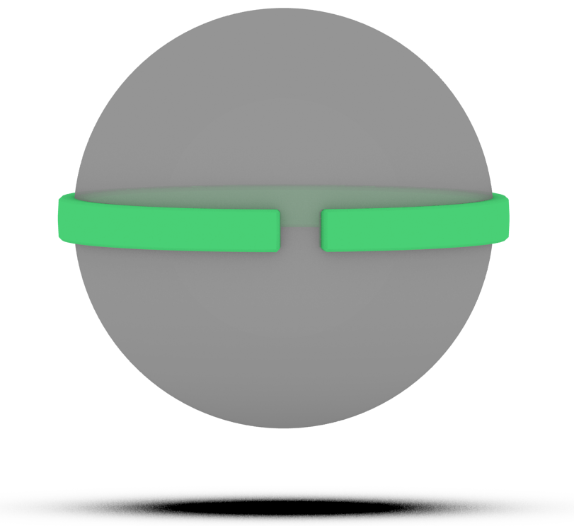
Let's define our state validity checker, which is a simple narrow band around the equator with a hole on one side:

bool obstacle(const ob::State *state)
{
    // As ob::ConstrainedStateSpace::StateType inherits from
    // Eigen::Map<Eigen::VectorXd>, we can grab a reference to it for some easier
    // state access.
    const Eigen::Map<Eigen::VectorXd> &x = *state->as<ob::ConstrainedStateSpace::StateType>();
 
    // Alternatively, we could access the underlying real vector state with the
    // following incantation:
    //   auto x = state->as<ob::ConstrainedStateSpace::StateType>()->getState()->as<ob::RealVectorStateSpace::StateType>();
    // Note the use of "getState()" on the constrained state. This accesss the
    // underlying state that was allocated by the ambient state space.
 
    // Define a narrow band obstacle with a small hole on one side.
    if (-0.1 < x[2] && x[2] < 0.1)
    {
        if (-0.05 < x[0] && x[0] < 0.05)
            return x[1] < 0;
 
        return false;
    }
 
    return true;
}
 
// Set the state validity checker in simple setup.
ss->setStateValidityChecker(obstacle);

Below, you can see a representation of this obstacle on our sphere.

Start and Goal

Now, let's also set the start and goal states, the south and north poles of the sphere. Note that for constrained problems, the start and goal states (if using exact states) must satisfy the constraint function. If they do not, then problems will occur.

// Start and goal vectors.
Eigen::VectorXd sv(3), gv(3);
sv << 0, 0, -1;
gv << 0, 0,  1;
 
// Scoped states that we will add to simple setup.
ob::ScopedState<> start(css);
ob::ScopedState<> goal(css);
 
// Copy the values from the vectors into the start and goal states.
start->as<ob::ConstrainedStateSpace::StateType>()->copy(sv);
goal->as<ob::ConstrainedStateSpace::StateType>()->copy(gv);
 
// If we were using an Atlas or TangentBundleStateSpace, we would also have to anchor these states to charts:
//   css->anchorChart(start.get());
//   css->anchorChart(goal.get());
// Which gives a starting point for the atlas to grow.
 
ss->setStartAndGoalStates(start, goal);

Planner

Finally, we can add a planner like normal. Let's use ompl::geometric::PRM, but any other planner in ompl::geometric would do.

auto pp = std::make_shared<og::PRM>(csi);

ss->setPlanner(pp);

Solving a Problem

With everything now in place, we can set everything up to get ready for planning:

ss->setup();

Same as how defining a problem is similar for constrained and unconstrained problems, solving a problem is also very similar. Let's give our planner 5 seconds of time and see what happens:

// Solve a problem like normal, for 5 seconds.
ob::PlannerStatus stat = ss->solve(5.);
if (stat)
{
    // Path simplification also works when using a constrained state space!
    ss->simplifySolution(5.);
 
    // Get solution path.
    auto path = ss->getSolutionPath();
 
    // Interpolation also works on constrained state spaces, and is generally required.
    path.interpolate();
 
    // Then do whatever you want with the path, like normal!
}
else
    OMPL_WARN("No solution found!");

Interpolation

Note that in general the initial path that you find is not "continuous". That is, the distance between states in the path (especially after simplification) can be very far apart! If you want a path that has close, intermediate constraint satisfying states, you need to interpolate the path. In the code above, this is achieved with ompl::geometric::PathGeometric::interpolate().

In Summary

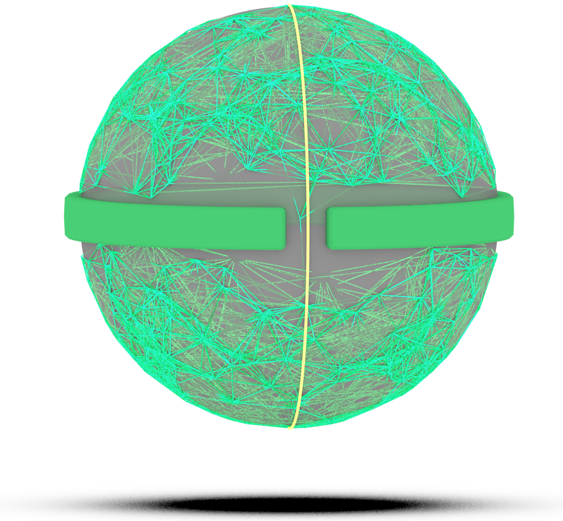
With all that, we've now solved a constrained motion planning problem on a sphere. A resulting motion graph for PRM could look something like this, with the simplified solution path highlighted in yellow:

Overall, planning with constraints is simple to setup and use. Beyond requiring you to define a constraint function and wrap your ambient space in a constrained state space, OMPL works and feels like normal. You can read more in general about constrained planning on the main page.

Table of Contents